Problem Statement

Buggy, also known as Sweepstakes, is a competition where Greek and independent organizations race with their buggies, small, low, aerodynamic vehicles, powered only by gravity and human pushers. At its fastest, a buggy can reach speeds up to 35 miles per hour. And yes - there’s a person in there!

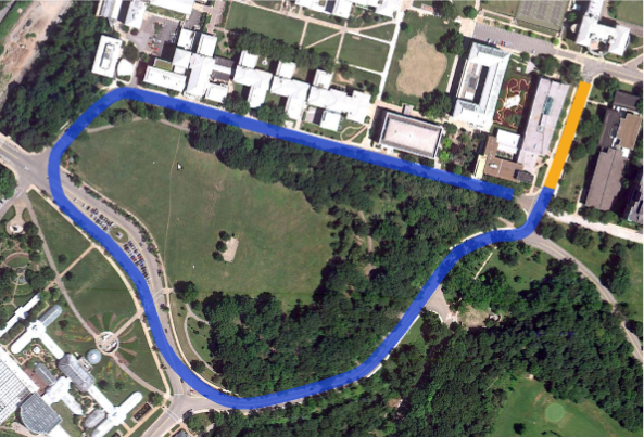
The objective of this project was to experiment with different forms of controllers for buggies not driven by humans. The buggies were modelled after the standard bicycle model. Lateral and Longitudinal dynamics were defined. A simulation platform was setup on Webots which accepted data from controllers designed by us.

Over the course of the project, we experimented with five different control schemes, each with increasing complexity and better returns than their predecessors.

Stage 1: PID Controllers

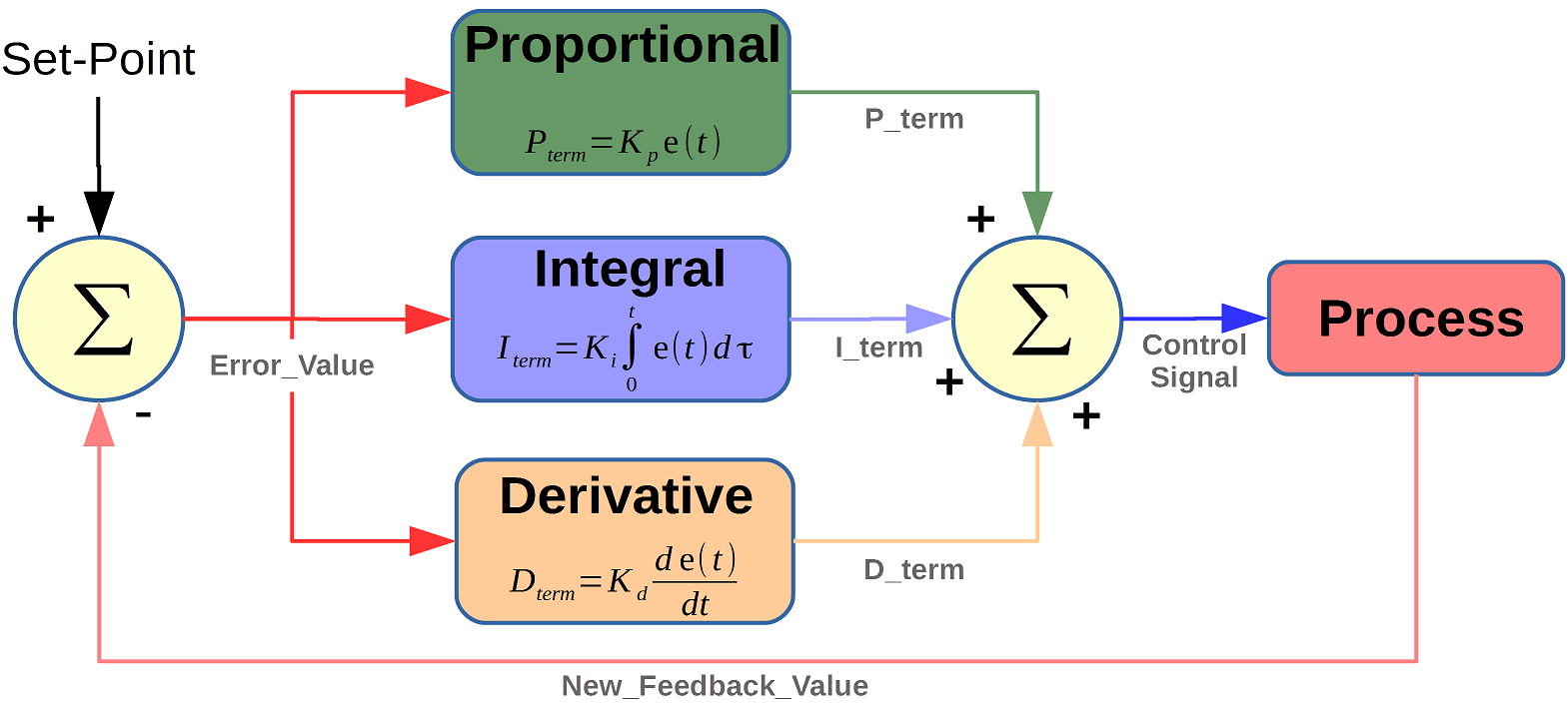
A PID controller is a key mechanism in industrial control systems, managing processes through three components: Proportional, Integral, and Derivative. The Proportional component generates an output proportional to the current error (the difference between the desired setpoint and the actual process variable), helping to reduce the error.

The Integral component tackles the steady-state error by accumulating the error over time, ensuring persistent errors are corrected, which helps bring the process variable closer to the setpoint.

The Derivative component predicts future error trends by considering the rate of change of the error, providing a damping effect that reduces overshoot and improves stability.

For our problem, the PID values were tuned for the longitudinal and lateral controllers, resulting in a laptime of 330 seconds. —–

Stage 2: State Feedback Controller With Pole Placement

A State Feedback Controller with Pole Placement is a control strategy used to achieve desired dynamic performance in control systems. It involves using the full state vector, which includes all the state variables of the system, to compute the control input. The control law typically takes the form ( u(t) = -Kx(t) + r(t) ), where ( u(t) ) is the control input, ( K ) is the state feedback gain matrix, ( x(t) ) is the state vector, and ( r(t) ) is the reference input. The objective is to design the gain matrix ( K ) so that the poles of the closed-loop system, which are the eigenvalues of the matrix ( A - BK ) (where ( A ) is the system matrix and ( B ) is the input matrix), are placed at specific locations in the s-plane (complex plane). These pole locations are chosen based on desired system characteristics such as stability, response time, and damping.

The design process involves determining the desired pole locations according to performance specifications and then computing the gain matrix ( K ) using methods like Ackermann’s formula or solving a set of linear equations. This approach allows for precise control over the system dynamics, enabling the designer to tailor the system’s performance to meet specific requirements. The main advantage of this method is its ability to provide exact control over the placement of the closed-loop poles, thereby ensuring the system behaves in a predictable and stable manner.

Our tuned controller saw a laptime of 200 seconds.

Stage 3: Linear Quadratic Controller

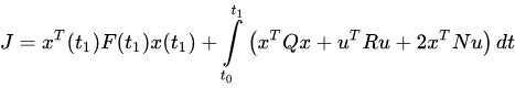
A Linear Quadratic Regulator (LQR) is an optimal control strategy used in linear systems to minimize a cost function, typically involving both state and control input variables. The goal of LQR is to find the control law u(t) = -Kx(t) that minimizes the quadratic cost function, where x is the state vector, u is the control input, Q is a positive semi-definite matrix weighting the state vector, and R is a positive definite matrix weighting the control input. By carefully choosing Q and R, designers can balance the trade-off between the performance of the system (keeping the states small) and the effort required (keeping the control inputs small).

The LQR design process involves solving the algebraic Riccati equation to find the optimal gain matrix K. This matrix K is then used to compute the control input that drives the system towards the desired performance. The primary advantage of LQR is its ability to systematically and optimally handle the trade-offs between state deviations and control efforts, ensuring a robust and efficient control system. LQR is widely used in various applications, including aerospace, robotics, and economics, due to its effectiveness and mathematical rigor.

The best LQR controller had a laptime of 120 seconds.

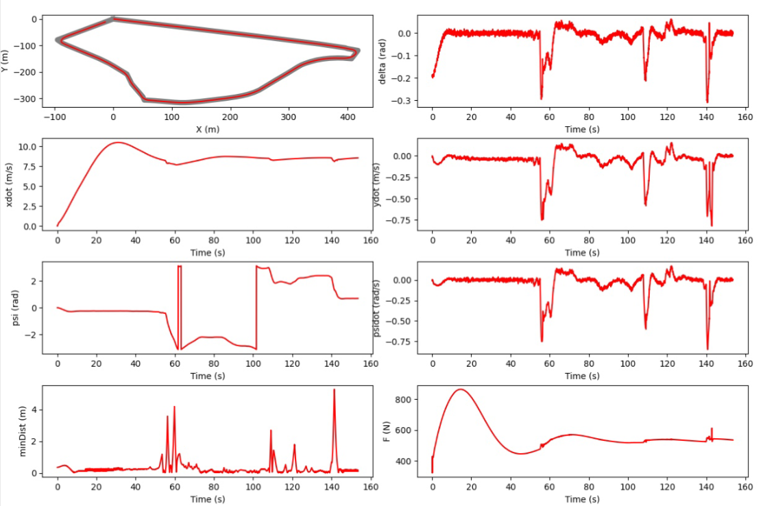
Stage 4: Model predictive Controller

A Model Predictive Controller (MPC) is an advanced control strategy that optimizes the control input by solving a finite horizon optimization problem at each time step. MPC uses a dynamic model of the system to predict future behavior over a specified prediction horizon. At each time step, the controller computes the control inputs by minimizing a cost function that typically includes terms for tracking error and control effort, subject to constraints on the inputs and states.

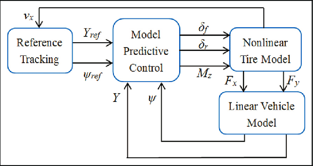
The main advantage of MPC is its ability to handle multi-variable control problems and incorporate constraints directly into the control design, making it suitable for complex industrial processes. By repeatedly solving the optimization problem as the system evolves, MPC can adjust the control inputs in real-time to account for changes and disturbances, ensuring optimal performance and robustness. This makes MPC widely used in process control, automotive applications, and energy management systems.

The best MPC controller had a laptime of 120 seconds.

Stage 5: Extended Kalman Filter Simultaneous Localization and Mapping

Extended Kalman Filter Simultaneous Localization and Mapping (EKF-SLAM) is a method used in robotics for building a map of an unknown environment while simultaneously keeping track of the robot’s location within that map. The Extended Kalman Filter (EKF) is an extension of the Kalman Filter that linearize the nonlinear models of the robot’s motion and sensor measurements, enabling it to handle the inherent nonlinearity in SLAM.

In EKF-SLAM, the state vector includes both the robot’s pose (position and orientation) and the locations of landmarks in the environment. The EKF uses the robot’s motion model to predict the state and the sensor measurements to update the state, reducing uncertainty over time. This approach ensures that the robot can navigate and map the environment accurately, even in the presence of noise and uncertainty. EKF-SLAM is widely used in autonomous navigation for applications like mobile robots, drones, and self-driving cars due to its effectiveness in real-time mapping and localization.

For the EKF SLAM the problem was compounded in terms of challenges. The best controller achieved a laptime of 160 seconds while managing the additional complexities.