Gaussian Splatting

Overview

In this project, we explore 3D Gaussian Splatting by building a simplified version of the 3D Gaussian rasterization pipeline introduced by the original paper. We create a rasterizer, use it to render pre-trained 3D Gaussians, and then optimize 3D Gaussians to represent custom scenes.

3D Gaussian Rasterization

We implement a 3D Gaussian rasterization pipeline in PyTorch. Our simplified implementation avoids many of the optimizations used by the official implementation for simplicity. We only use the view independent components of the spherical harmonic coefficients.

Project 3D Gaussians to Obtain 2D Gaussians

We project 3D Gaussians in the world space to 2D Gaussians on the image plane of a camera. Following equations (5) and (6) of the original paper, we obtain a 2D Gaussian that represents an approximation of the projection of a 3D Gaussian.

Filter and Sort Gaussians

Before starting the rasterization procedure, we sort the 3D Gaussians in increasing order by their depth value and discard 3D Gaussians whose depth value is less than 0.

Compute Alphas and Transmittance

Using the ordered and filtered 2D Gaussians, we compute their alpha and transmittance values at each pixel location in an image.

Perform Splatting

Using the computed alpha and transmittance values, we blend the color value of each 2D Gaussian to compute the color at each pixel.

We also compute the depth and silhouette (mask) maps.

After implementing the rasterizer, we test it by rendering views of a scene represented by pre-trained 3D Gaussians. Here is one frame of the GIF output:

Training 3D Gaussian Representations

We use our 3D Gaussian rasterizer to train a 3D representation of a scene given posed multi-view data. We train a 3D representation of a toy cow using isotropic Gaussians.

Setting Up Parameters and Optimizer

We make the 3D Gaussian parameters trainable and set up the optimizer with different learning rates for each type of parameter.

Perform Forward Pass and Compute Loss

We render the 3D Gaussians to predict an image rendering viewed from a given camera and implement a loss function that compares the predicted image rendering to the ground truth image.

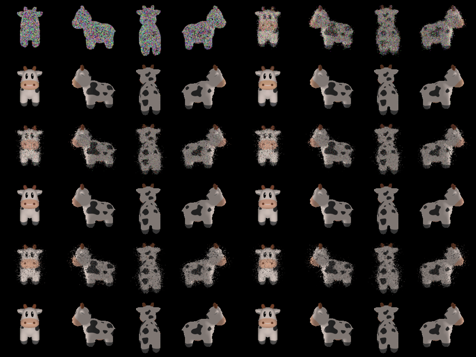
After training, we obtain the following training progress GIF:

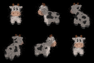
And the final rendering GIF:

Extensions

Rendering Using Spherical Harmonics

We explore rendering 3D Gaussians with associated spherical harmonic components to model view-dependent effects. We modify the code to enable the utilization of spherical harmonics and render views of a scene represented by pre-trained 3D Gaussians.

Training On a Harder Scene

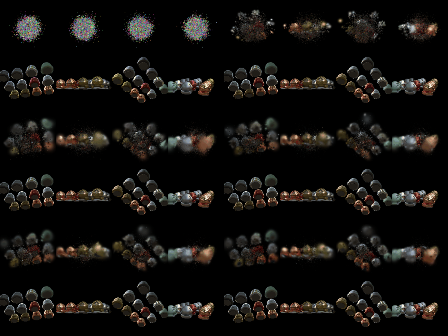
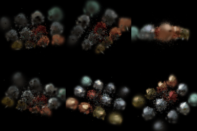
We train 3D Gaussians on a more challenging scene with randomly initialized points for the 3D Gaussian means. We experiment with techniques to improve performance, such as different learning rates, learning rate scheduling, SSIM loss, adaptive density control, initialization parameters, and using anisotropic Gaussians.

Conclusion

This project demonstrates the implementation and application of 3D Gaussian Splatting for representing and rendering 3D scenes. We build a simplified 3D Gaussian rasterizer, render pre-trained 3D Gaussians, and optimize 3D Gaussians to represent custom scenes. We also explore extensions such as rendering with spherical harmonics and training on harder scenes.